Bertrand’s Paradox - Owen Medeiros

Bertrand’s paradox is a problem within the classical interpretation of probability theory, first posed by Joseph Bertrand in 1889. It shows how different methods of selecting a “random” chord in a circle can yield different probabilities for the same question.

The Problem¶

Given a circle, what is the probability that a randomly chosen chord is longer than the side of an inscribed equilateral triangle?

Three Different Approaches¶

The paradox demonstrates that this seemingly simple question has three different answers depending on how we interpret “random”:

Random endpoints: Choose two random points on the circle’s circumference
Random radial distance: Fix one endpoint and choose the other randomly
Random midpoint: Choose the chord’s midpoint randomly within the circle

Each method gives a different probability: 1/3, 1/2, and 1/4 respectively.

MATLAB Simulation¶

The following MATLAB code demonstrates all three approaches with visual simulation:

radius = 2;
close all

N = 1000;
angles = linspace(0,360, N);
CenterX = 0;
CenterY = 0;
x = radius .* cos(angles) + CenterX;
y = radius .* sin(angles) + CenterY;

subplot(3,1,1)
hold on
c1 = [103 103 100]./255;  % Shorter chords (brown)
c2 = [247 153 113]./255;  % Longer chords (orange)

% Method 1: Random endpoints
for i = 1:N
    r1 = randi(N);
    r2 = randi(N);

    p1(i,:) = [x(r1) y(r1)];
    p2(i,:) = [x(r2) y(r2)];

    midpoint(i,:) = [(p1(i,1)+p2(i,1))/2 (p1(i,2)+p2(i,2))/2];
    
    % Check if chord is longer than triangle side
    if (midpoint(i,1)-CenterX)^2+(midpoint(i,2)-CenterY)^2>(radius/2)
        carray(i,:) = c1;  % Shorter chord
    else
        carray(i,:) = c2;  % Longer chord
    end
end

% Plot sample of chords
for i = 1:100
    plot([p1(i,1) p2(i,1)], [p1(i,2) p2(i,2)], 'Color', carray(i,:));
    hold on
end
axis equal
axis off
title('Method 1: Random Endpoints (P = 1/3)')

% Method 2: Fixed endpoint, random other point
subplot(3,1,2)
a = radius*3/sqrt(3);

for i = 1:N
    r1 = randi(N);
    
    p1(i,:) = [CenterX CenterY-radius];  % Fixed bottom point
    p2(i,:) = [x(r1) y(r1)];            % Random point on circle

    % Check if chord is longer than triangle side
    if x(r1) > -a/2 && x(r1) < a/2 && y(r1) > radius/2
        carray(i,:) = c2;  % Longer chord
    else
        carray(i,:) = c1;  % Shorter chord
    end
end

% Plot sample of chords
for k = 1:100
    i = randi(N);
    plot([p1(i,1) p2(i,1)], [p1(i,2) p2(i,2)], 'Color', carray(i,:));
    hold on
end
axis equal
axis off
title('Method 2: Fixed Endpoint (P = 1/2)')

% Method 3: Random midpoint
subplot(3,1,3)

for i = 1:N
    r1 = randi(N);
    
    p1(i,:) = [x(r1) y(r1)];
    p2(i,:) = [-x(r1) y(r1)];  % Symmetric chord

    % Check if chord is longer than triangle side
    if abs(y(r1)) > radius/2  
        carray(i,:) = c2;  % Longer chord
    else
        carray(i,:) = c1;  % Shorter chord
    end
end

% Plot sample of chords
for k = 1:100
    i = randi(N);
    plot([p1(i,1) p2(i,1)], [p1(i,2) p2(i,2)], 'Color', carray(i,:));
    hold on
end
axis equal
axis off
title('Method 3: Random Midpoint (P = 1/4)')

Visualization¶

The simulation generates three subplots showing each method, with chords colored by length:

Brown: Chords shorter than the triangle side
Orange: Chords longer than the triangle side

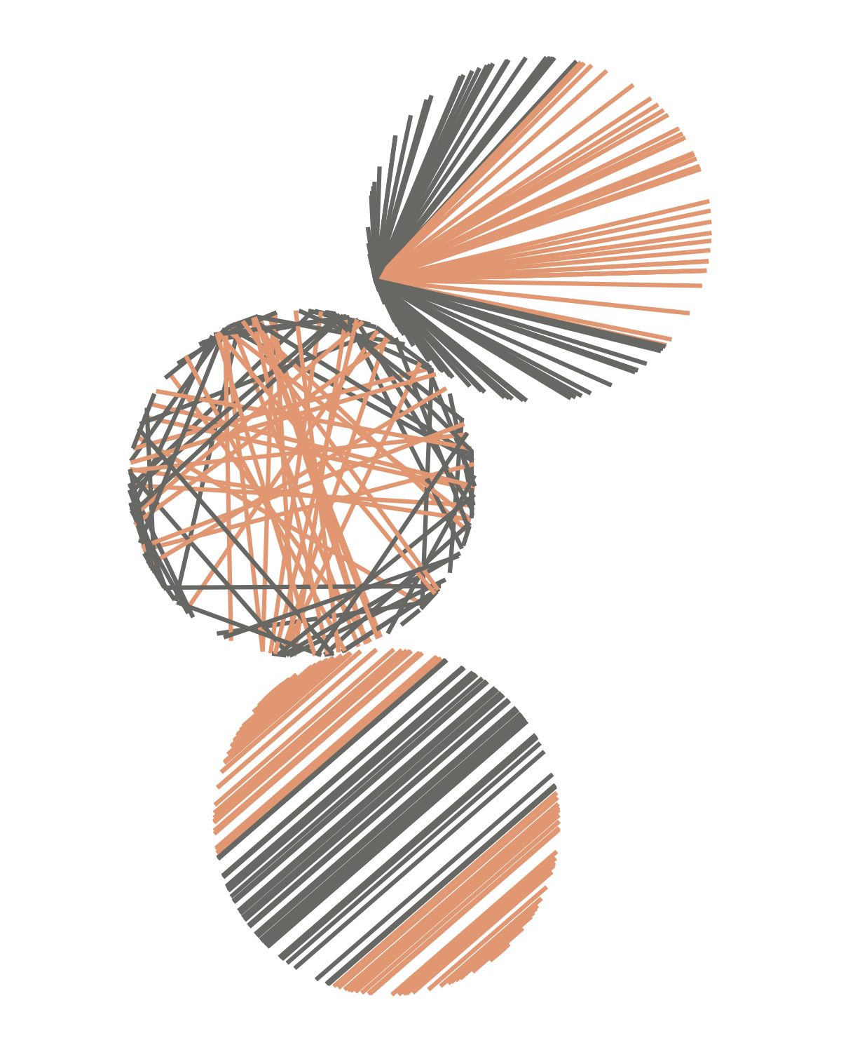
Figure 1:Visual comparison of the three different interpretations of Bertrand’s Paradox. Each panel shows 100 sample chords colored by their length relative to an inscribed equilateral triangle.

Download MATLAB Code